Forest Fire Detection using CNN - Part 2

In this article we'll see more in-depth about the Part 1 of this project.

If you haven't seen Part 1, head over to Forest Fire Detection using CNN Part 1

Dataset Link:

https://www.kaggle.com/datasets/brsdincer/wildfire-detection-image-data

Code on GitHub repo: https://github.com/Mayuresh999/Projects/tree/main/Forest%20Fire%20Detection%20using%20CNN

Code on Kaggle:

https://www.kaggle.com/code/mayureshnm/forest-fire-detection-using-cnn

CNN ( Convolutional Neural Network )

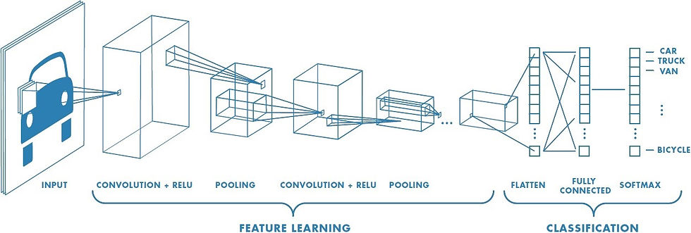
The model used in Part 1 is exactly same as the above image. Just the last layer in our case uses Sigmoid activation function instead of Softmax. This is because Sigmoid is the activation function that gives binary output and we exactly need that to happen as we only have two outputs i.e. "Fire" or "NoFire". Sigmoid on the other hand gives multiple outputs depending on the output we expect. To know more about "Activation Functions" refer the previous article on the same topic Activation Functions in brief.

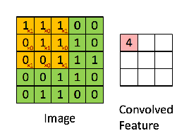
I brief, CNN works by multiplicating the matrix of Input Image to the Filter to see the details and learn the patterns. Pictorial representation helps us understand this better.

Prerequisites

• Google Colab

I have used Google Colab as it has TPU. Tensor Processing Unit has helped me a lot to cut down the training time significantly. Prior to that, I tried using GPU but that was a bit slow.

Input Image Dataset

The dataset is available on Kaggle. Dataset contains two folders namely "Testing" and "Training and Validation". Both of these folders have subfolders naming "Fire" and "NoFire". In training dataset there are 150 samples of images each target variable and testing dataset contains 50 samples each. I have stored the file on my Drive for easy access to Google Colab.

Importing Libraries

I have imported following libraries

import tensorflow as tf
import numpy as np
from tensorflow import keras
import os
import cv2
from tensorflow.keras.preprocessing.image import ImageDataGenerator
from tensorflow.keras.preprocessing import image
import matplotlib.pyplot as plt

Making separate datasets for training and testing

To access the files easily we have to make separate datasets. I've done so by first rescaling the images to 1/255 so that the array will have values between 0 and 1 as it is important step to be done. Then using flow_from_directory method from keras, which takes a path of a directory and generates batches of augmented data, we have smooth connectivity with the data to the model. Target size is important because real-world images can be in different size so what ever the input image size be it will be resized to 150X150 image. Then we specify batch size which simply means the number of samples that will be propagated through the network in a given time 32 is the default value for that function. Then here our classification result fall in one of the two classes i.e. Fire or NoFire hence we specify class_mode as binary.

train = ImageDataGenerator(rescale=1/255)
test = ImageDataGenerator(rescale=1/255)

train_dataset = train.flow_from_directory("/content/drive/MyDrive/forest_fire/Training and Validation/",target_size=(150,150),batch_size = 32,class_mode = 'binary')

test_dataset = test.flow_from_directory("/content/drive/MyDrive/forest_fire/Testing/",target_size=(150,150),batch_size =32,class_mode = 'binary')

Model Building

Keras has an useful API which makes us easier to define the layers of our neural network. We have put the input_shape as 150,150 which is our image size and 3 represents color channel RGB. If it is a gray scale image the we should specify it as 1.

• Conv2D() : Neural networks apply a filter to an input image to create a feature map that summarizes the presence of detected features in the input. In our case there are 32,64,128 and 128 filters or kernels in respective layers and the size of the filters are 3X3 with activation functions as ReLU.

• MaxPool2D() :Max pooling is a pooling operation that selects the maximum element from the region of the feature map covered by the filter. Thus, the output after max-pooling layer would be a feature map containing the most prominent features of the previous feature map.

• Flatten() : This method converts the multi-dimensional image data array to 1D array.

model=keras.Sequential()

# Convolutional layer and maxpool layer 1

model.add(keras.layers.Conv2D(32,(3,3),activation='relu', input_shape=(150,150,3)))
model.add(keras.layers.MaxPool2D(2,2))

# Convolutional layer and maxpool layer 2

model.add(keras.layers.Conv2D(64,(3,3), activation='relu'))
model.add(keras.layers.MaxPool2D(2,2))

# Convolutional layer and maxpool layer 3

model.add(keras.layers.Conv2D(128,(3,3), activation='relu'))
model.add(keras.layers.MaxPool2D(2,2))

# Convolutional layer and maxpool layer 4

model.add(keras.layers.Conv2D(128,(3,3), activation='relu'))
model.add(keras.layers.MaxPool2D(2,2))

# This layer flattens the resulting image array to 1D array

model.add(keras.layers.Flatten())

# Hidden layer with 512 neurons and Rectified Linear Unit activation function 

model.add(keras.layers.Dense(512, activation='relu'))

# Output layer with single neuron which gives 0 for Fire or 1 for NoFire 
# Here we use sigmoid activation function which makes our model output to lie between 0 and 1

model.add(keras.layers.Dense(1, activation='sigmoid'))

Compiling the model

After this we have to specify an optimizer and a loss function for our model and also metrics which we want to visualize while training. The role of optimizer is it measure how good our model predicted output when compared with true output if the loss is high then Optimizers are used to change the attributes of your neural network such as weights and learning rate in order to reduce the losses. There are several optimizers and loss functions available in TF. Here we use adam and binary_crossentropy. If it was a multi-class classification then we use sparse_categorical_crossentropy as loss function. To know more on Optimizers, you can see the article I have made earlier Optimization Methods in Deep Learning.

model.compile(optimizer='adam',loss='binary_crossentropy',metrics=['accuracy'])

Fitting the model

We can train our mode by calling fit() function which takes our training images and also our validation images as input for training and also for validation. Also we should specify epochs and steps per epoch. The most common way to choose steps per epoch is the ratio of number of train images to the batch size. In our case it is 45 which is decided by the model automatically. I have saved the fit function in a variable "r" so that we can see the performance of model on a graph.

It takes some time to train the model depending upon no of layers, Data-set size etc. Hence I have used TPU as hardware accelerator as it sped up the training process a lot. This is the main reason I've used Google Colab for this project instead of regular Jupyter notebook as my system does not have any hardware accelerator.

r = model.fit(train_dataset,epochs = 10,validation_data = test_dataset)

Predicting on Test Dataset

Here we have predicted the values on Test dataset to see the values. It shows an array of 0 and 1 which is as expected.

predictions = model.predict(test_dataset)
predictions = np.round(predictions)
predictions

Plotting loss per iteration

We have fitted the model and now we can see how it performed in the process by plotting the graph of 'loss' and 'validation loss' vs 'iterations'. The graph shows that the model has just performed satisfactorily and it can be further improved.

import matplotlib.pyplot as plt
plt.plot(r.history['loss'], label='loss')
plt.plot(r.history['val_loss'], label='val_loss')
plt.legend()

Plotting accuracy per iteration

We can also see the graph of 'accuracy' and 'validation accuracy' vs 'iterations'. This also shows that the model can be made more better predictor using further advanced methods.

plt.plot(r.history['accuracy'], label='acc')
plt.plot(r.history['val_accuracy'], label='val_acc')
plt.legend()

Making a function to see any image from dataset with predicted label

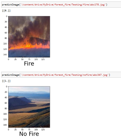
Here we have a simple function which takes filename of the image (along with path) as input then load it using load_image method of keras. After this it will resize the image as 150X150 and plot it using matplotlib, convert it into a numpy array then expand the dimension of that array and store it in another variable X. Then it passes it as an input to predict method of model object. It returns a value which lies between 0 and 1 due to sigmoid activation function in output layer. Then if the value is 1, X axis label is set as "Fire". If it is 0, then X axis label is set as "No Fire".

Now call the function by passing the path of the image.

def predictImage(filename):
    img1 = image.load_img(filename,target_size=(150,150))
    plt.imshow(img1)
    Y = image.img_to_array(img1)
    X = np.expand_dims(Y,axis=0)
    val = model.predict(X)
    print(val) 
    if val == 1:
        plt.xlabel("No Fire",fontsize=30)
    elif val == 0:
        plt.xlabel("Fire",fontsize=30)

Following are some images the Model predicted correctly.

Predicting images from Google

I also wanted to see if the model is actually good enough to predict the images outside of dataset. So I downloaded some images from Google and tried predicting those. To do this, I had to download those and store them in my Google Drive because directly giving the web link to the model didn't work. The prediction was kind of satisfactory as sometimes it predicted "NoFire" even though the image showed fire in the forest.

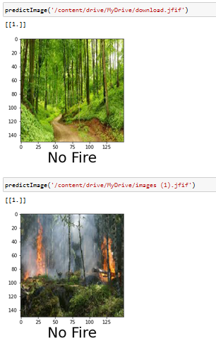
Above are some images from the internet which supposedly do not exist in the dataset.

Future Ideas

I will try to make a Part 3 for this and improve the model further more using Transfer Learning technique and more Hyperparameter tuning.

. . .

Like , Share if you found this helpful.

I am open to any Suggestions/ Corrections/ Comments so please feel free.

Also , Connect with me on Linkedin

Open to Entry Level Jobs/ Internships as Data Scientist/Data Analyst. Please DM on Linkedin for my Resume for any openings in near future 🤗 🙏