Do It Yourself Deep Learning Projects
- Mayuresh Madiwale
- Aug 14, 2022
- 6 min read

In this post we'll see all the steps that will help you create your own Deep Learning Project. This post will serve as a roadmap with everything that you'll need right from dataset importing to model saving. It would be great if you try it yourself and post the link of your project in the comments.
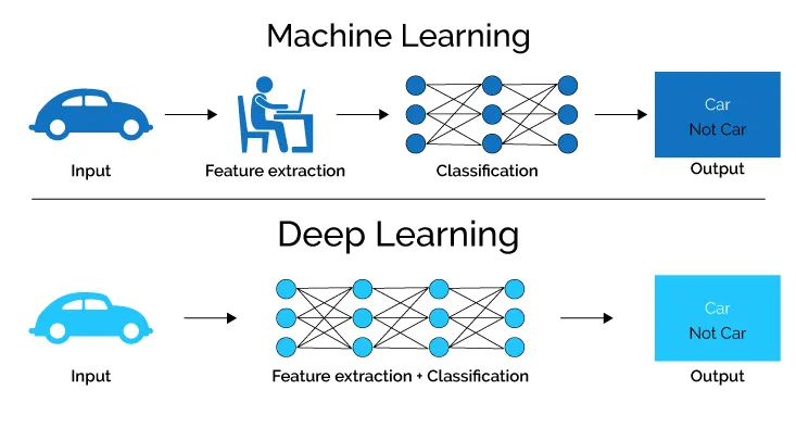
Deep Learning is a branch of Data Science which handles all the big stuff such as large datasets of all types of data. whether be it numerical, textual or images. This post will specifically cover the image classification with Transfer Learning process which uses CNN models. You can refer the other previous articles around the same topic at the end of this post.
The Dataset
There are plenty of datasets available on online platforms such as Kaggle, GitHub, TensorFlow Datasets, Keras Datasets, etc. You can either import datasets from above sources directly to your notebook using links such as Kaggle API method, GitHub Cloning method (More on it Here) or you can manually download it in your local system. Again Kaggle and GitHub are some of the most famous platforms to download image datasets.
Test, Validation and Train Split
This method will help you organize the data if the dataset doesn't already have splits made. I have faced this issue and found a wonderful library that will split the dataset to train, validation and test folders on specified ratio and create separate folders in your local system.
import splitfolders

splitfolders.ratio('path to the input folder',
    output = "path to the output folder",
    seed = 'any random number e.g. (1000)',
    ratio= 'ratio of split as per your choice in the format (train, test,
    validation) e.g.(.8, 0.1,0.1)')
If you don't have the library installed, you can refer about it Here
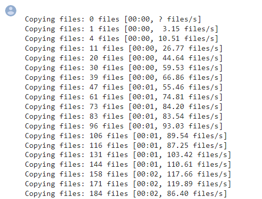
Output of above code will be as following.

After this there will be three folders made in your local system at the provided output path. From here you can visualize some samples in your notebook after importing the train, test and validation dataset.
Importing the dataset in Notebook
There are two ways from which you can import the datasets in the notebook.
ImageDataGenerator with flow_from_directory
TensorFlow Keras Preprocessing with image_dataset_from_directory
ImageDataGenerator Flow From Directory is great as it can pass the data from either local system or GDrive if you are using Colab. Both of the above processes are available in Keras Preprocessing. In ImageDataGenerator you can put arguments to augment the data beforehand. So if you want to do Data Augmentation right when you import the data, you can use this method. Code snippet is as follows.
train = ImageDataGenerator(rescale = 1/255, rotation_range = 40,
                                          horizontal_flip = True,
                                          width_shift_range = 0.2,
                                          height_shift_range = 0.2,
                                          shear_range = 0.2,
                                          zoom_range = 0.2,
                                          fill_mode = 'nearest')

train_dataset = train.flow_from_directory('input folder path',
                                          target_size = (224,224),
                                          batch_size = 32,
                                          seed = 1000,
                                          class_mode = 'categorical')
Here you can input the rescaling as it is important for model to learn. CNN can only take value of images that are between 0 and 1. After this you can pass whatever augmentation you might want in the ImageDataGenerator block and then pass the variable to the flow_from_directory where you specify the input folder, target size, batch size, seed, class mode and other arguments. target size is an important parameter as the pre trained models specify what input size the want and we have to provide the correct size. class mode can be either "categorical" or "binary".
Image Dataset from Directory is also a fast and reliable method to import datasets in your notebook. This has an added advantage that will help you a lot in the later part. Here you will have to augment the images separately as this function is not available in the function. Code snippet is as follows.
train_data = tf.keras.preprocessing.image_dataset_from_directory("input path",
    seed = 123,
    shuffle = True,
    image_size = (224,224),
    batch_size = 32)
In the above code you have to give the input folder path followed by the other arguments such as shuffle, image and batch size.
Visualize a Sample of your Data
After importing the dataset we can view some samples in the notebook. This is the part where the second image importing method (Image Dataset from Directory) comes handy. The dataset is large and we only want to see some samples randomly from different classes, here, there is a function in the second method that will pick up the images randomly and then we can view it.
Firstly we will make a variable to store the class names of dataset. This can be easily done using following code example.
class_names = train_dataset.class_namesThen we will make a user defined function to make a subplot of samples. example is as follows.
plt.figure(figsize=(10, 10))
for image_batch, labels_batch in train_dataset.take(1):
    for i in range(12):
        ax = plt.subplot(3, 4, i + 1)
        plt.imshow(image_batch[i].numpy().astype("uint8"))
        plt.title(class_names[labels_batch[i]])
        plt.axis("off")
In above example I have made a 10 by 10 grid to plot images in which train_dataset.take(1) will take 1 sample of batch size 32. The output will be a grid of 12 images with the class name as title.
Importing the Pre-Trained Model
There are many platforms that offer free pre trained models as discussed in the last post (see them Here). Follow the steps as instructed on the platform and then you'll be able to successfully import the model. Before that you will have to do the importing of required libraries as shown in the code example below.
from tensorflow.keras.layers import Input, Lambda, Dense, Flatten
from tensorflow.keras import models, layers
from tensorflow.keras.models import Model
from tensorflow.keras.applications.inception_v3 import InceptionV3
from tensorflow.keras.applications.inception_v3 import preprocess_input
from tensorflow.keras.preprocessing import image
from tensorflow.keras.preprocessing.image import ImageDataGenerator,load_img
from tensorflow.keras.models import Sequential
Here, I have used Inception V3 model from Keras. Now we will do the hyperparameter tuning for the same model.
inception = InceptionV3(input_shape=[224,224,3], weights="imagenet", include_top=False)
x = Flatten()(inception.output)
Here, the weights are the most important parameter that will decide the accuracy of your model. This model is trained on ImageNet Dataset hence, the weights are set to that. If you want only the model architecture without pre trained weights, you can set it to None. Include Top will include the classes that were used in training. we have a separate dataset so we will not include the top layers. Finally we will predict the images from test dataset after fitting the model.
Fitting the Model
In this step we will transfer the intelligence (weights) of our pre trained model for solving our case, hence the name transfer learning. Code snippet below will ease our understanding.
prediction = Dense(len(class_names), activation='softmax')(x)

model = Model(inputs=inception.input, outputs=prediction)

model.compile(
  loss=tf.keras.losses.SparseCategoricalCrossentropy(from_logits=False),
  optimizer='adam',
  metrics=['accuracy'])

history = model.fit(
    train_data,
    batch_size=32,
    validation_data=val_data,
    verbose=1,
    epochs=10)
In above code, we have made the last layer of model as dense layer with the number of neurons same as the length of classes in our data. We have used SoftMax Activation function to get probability value of the classes. In compiling, we have specified our metrices of model evaluation such as loss and accuracy metric and our optimizer as "Adam". Finally, in fitting of our model we passed our data, batch size and validation data along with number of epochs we want. The output will show as fitting process. You can reduce the time by using GPU or TPU that are available in Google Colab.

Evaluate the Model on Test Data
In this phase, we will evaluate how the model performed over the epochs and also see the predictions. To see the validation accuracy and train accuracy over time, we will make a function as follows.
plt.plot(history.history['accuracy'], label='accuracy')
plt.plot(history.history['val_accuracy'], label='val_accuracy')
plt.legend()
Similarly to see the loss, we will make another function as follows.
plt.plot(r.history['loss'], label='loss')
plt.plot(r.history['val_loss'], label='val_loss')
plt.legend()
Visualize the Predicted Results with Confidence
To see the model prediction and confidence of model to predict the outputs, we will have to make two functions that will help us achieve our goal.
def predict(model, img):
    img_array = tf.keras.preprocessing.image.img_to_array(images[i].numpy())
    img_array = tf.expand_dims(img_array, 0)

    predictions = model.predict(img_array)

    predicted_class = class_names[np.argmax(predictions[0])]
    confidence = round(100 * (np.max(predictions[0])), 2)
    return predicted_class, confidence
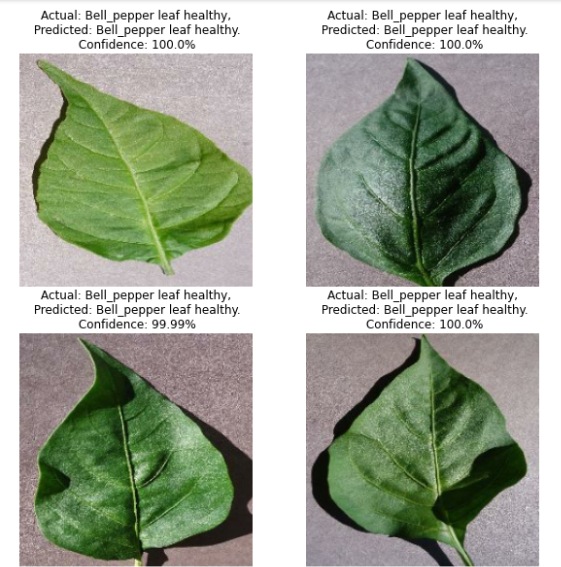
This function will make the predictions and place them in a variable predicted_class and give the confidence value in percent and place them in variable named confidence
After this we will make another function to plot the images.
plt.figure(figsize=(10, 10))
for images, labels in test_dataset.take(1):
    for i in range(4):
        ax = plt.subplot(2, 2, i + 1)
        plt.imshow(images[i].numpy().astype("uint8"))
        predicted_class, confidence = predict(model, images[i].numpy())
        actual_class = class_names[labels[i]]
        plt.title(f"Actual: {actual_class},\n Predicted:         {predicted_class}.\n Confidence: {confidence}%")
        plt.axis("off")
output of above code will be as follows.

Model Saving
Saving the model will give us the only file we require to predict any image in future. Also this will help us to deploy our model on some cloud if we want to make a web app or any on-device app. It is pretty simple to save a model.
model.save("../"model name".h5")You will have to give the path where you want to save it.
Yay!! You have done it!.
Post the notebook in you GitHub and Mention it wherever you like. Comment the link to your project in the comment section of this Linkedin post to let others know about your project.
Final Thoughts
There might be many other advanced techniques that are involved in complete end to end project. but this post will set your understandings and give you path to make a basic image classifier.
If you are a beginner in the field, you can make as many projects as you want and showcase them in your resume.
. . .
Like , Share if you found this helpful.
I am open to any Suggestions/ Corrections/ Comments so please feel free.
Also , Connect with me on Linkedin 🤗 🙏


Comments