Forest Fire Detection using CNN Part 4
- Mayuresh Madiwale
- Jul 18, 2022
- 5 min read

In this article we'll see more in-depth about the Part 3 of this project.
If you haven't seen Part 1 & 2, head over to:
We have already discussed about the prerequisites of the project and brief about the CNN working in part 2, so lets drive to the main points.
Importing Libraries
import tensorflow as tf
import numpy as np
from tensorflow import keras
import os
import cv2
import tensorflow_hub as hub
from tensorflow.keras.preprocessing.image import ImageDataGenerator
from tensorflow.keras.preprocessing
import image
import matplotlib.pyplot as plt
Making separate datasets for training and testing
To access the files easily we have to make separate datasets. I've done so by first rescaling the images to 1/255 so that the array will have values between 0 and 1 as it is important step to be done.
Then using flow_from_directory method from keras, which takes a path of a directory and generates batches of augmented data, we have smooth connectivity with the data to the model.
Target size is important because real-world images can be in different size so what ever the input image size be it will be resized to 224X224 image.
Then we specify batch size which simply means the number of samples that will be propagated through the network in a given time 32 is the default value for that function.
Then here our classification result fall in one of the two classes i.e. Fire or NoFire hence we specify class_mode as binary.
train = ImageDataGenerator(rescale=1/255)
test = ImageDataGenerator(rescale=1/255)

train_dataset = train.flow_from_directory("/content/drive/MyDrive/forest_fire/Training and Validation/",target_size=(224,224),batch_size = 32,class_mode = 'binary')

test_dataset = test.flow_from_directory("/content/drive/MyDrive/forest_fire/Testing/",target_size=(224,224),batch_size =32,class_mode = 'binary')
Importing the Model
feature_extractor_model = "https://tfhub.dev/google/tf2-preview/mobilenet_v2/feature_vector/4"

pretrained_model_without_top_layer = hub.KerasLayer(feature_extractor_model, input_shape=(224, 224, 3), trainable=False)
Loading the model
Here we have the link of the model from TensorFlow Hub saved in the variable named feature_extractor_model.
Then we have put that into the KerasLayer with input shape as 224 x 224 x 3. here the model requires this specific shape by default, so there's hardly anything to do in the input shape.
Trainable = False means we have stopped the model training and we only need it's weights and biases that are already included in the pretrained model. This is a hyperparameter.
In the last step we have added 1 single neuron to predict within the range of 0 and 1 i.e. "Fire" or "NoFire" respectively. To do this "Sigmoid" is the perfect Activation Function.
model = tf.keras.Sequential([pretrained_model_without_top_layer,tf.keras.layers.Dense(1,activation='sigmoid' )])

model.summary()
Compiling the model
After this we have to specify an optimizer and a loss function for our model and also metrics which we want to visualize while training. The role of optimizer is it measure how good our model predicted output when compared with true output if the loss is high then Optimizers are used to change the attributes of your neural network such as weights and learning rate in order to reduce the losses.
There are several optimizers and loss functions available in TF. Here we use adam and binary_crossentropy. If it was a multi-class classification then we use sparse_categorical_crossentropy as loss function. To know more on Optimizers, you can see the article I have made earlier Optimization Methods in Deep Learning.
model.compile(optimizer="adam",loss='binary_crossentropy',metrics=['accuracy'])Fitting the model
We can train our mode by calling fit() function which takes our training images and also our validation images as input for training and also for validation.
Also we should specify epochs and steps per epoch. The most common way to choose steps per epoch is the ratio of number of train images to the batch size. In our case it is 45 which is decided by the model automatically.
I have saved the fit function in a variable "r" so that we can see the performance of model on a graph.
It takes some time to train the model depending upon Data, Model, Data-set size etc. Hence I have used TPU as hardware accelerator as it sped up the training process a lot. This is the main reason I've used Google Colab for this project instead of regular Jupyter notebook as my system does not have any hardware accelerator.
Early Stopping is a miracle of Deep Learning. This is a function which monitors the model performance and stops the further iterations if the monitored value is repeating for "n" number of times. The "n" is decided by us and is called "patience".
callback = tf.keras.callbacks.EarlyStopping(monitor='loss', patience=3)

r = model.fit(train_dataset, epochs=10, validation_data = test_dataset, callbacks=[callback] )
Predicting on Test Dataset
Here we have predicted the values on Test dataset to see the values. It shows an array of 0 and 1 which is as expected.
predictions = model.predict(test_dataset)predictions = np.round(predictions)Plotting loss per iteration
We have fitted the model and now we can see how it performed in the process by plotting the graph of 'loss' and 'validation loss' vs 'iterations'.
plt.plot(r.history['loss'], label='loss')
plt.plot(r.history['val_loss'], label='val_loss')
plt.legend()
Plotting accuracy per iteration
We can also see the graph of 'accuracy' and 'validation accuracy' vs 'iterations'.
plt.plot(r.history['accuracy'], label='acc')
plt.plot(r.history['val_accuracy'], label='val_acc')
plt.legend()
Making a function to see any image from dataset with predicted label
Here we have a simple function which takes filename of the image (along with path) as input then load it using load_image method of keras.
After this it will resize the image as 224 X 224 and plot it using matplotlib, convert it into a numpy array then expand the dimension of that array and store it in another variable X.
Then it passes it as an input to predict method of model object.
It returns a value which lies between 0 and 1 due to sigmoid activation function in output layer.
Then if the value is 1, X axis label is set as "Fire".
If it is 0, then X axis label is set as "No Fire".
Now call the function by passing the path of the image.
def predictImage(filename):
    img1 = image.load_img(filename,target_size=(224,224))
    plt.imshow(img1)
    Y = image.img_to_array(img1)
    X = np.expand_dims(Y,axis=0)
    val = model.predict(X)
    val = np.round(val)
    print(val)
    if val == 1:
        plt.xlabel("No Fire",fontsize=30)
    elif val == 0:
        plt.xlabel("Fire",fontsize=30)
predictImage('/content/drive/MyDrive/forest_fire/Training and Validation/nofire/abc218.jpg')With this we have completed all the steps for Transfer Learning. Now let's analyze our results.
Model 1 Name :- tf2-preview/mobilenet_v2/feature_vector
[TF2] Feature vectors of images with MobileNet V2 trained on ImageNet (ILSVRC-2012-CLS).
Publisher: Google
License: Apache-2.0
Architecture: MobileNet V2 Dataset: ImageNet (ILSVRC-2012-CLS)
Read more about it Here.
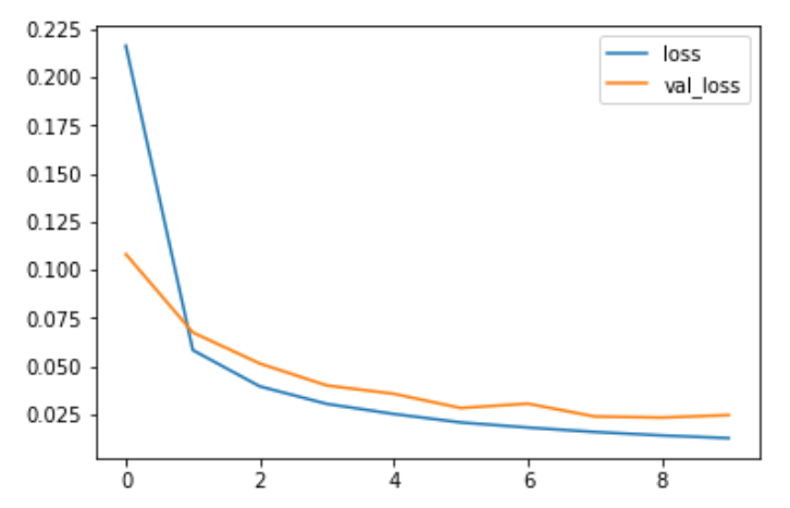
Loss per Iteration plot
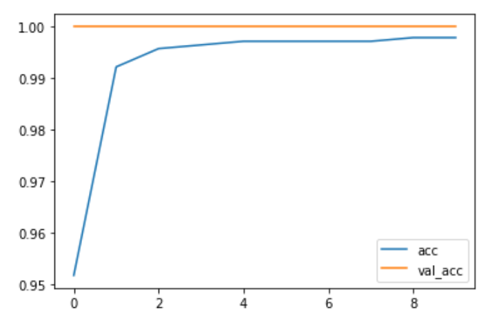
Accuracy per Iteration plot
Looks great isn't it? ....
Well!!!
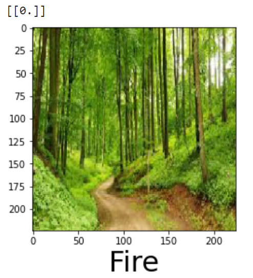
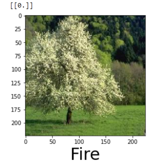
That's not going to work. Let's use different model and try our luck.
Model 2 Name : - imagenet/efficientnet_v2_imagenet21k_ft1k_b0/classification
Imagenet (Full ImageNet, Fall 2011 release) classification with EfficientNet V2 with input size 224x224. Fine-tuned on ImageNet1K.
Publisher: Google
License: Apache-2.0
Architecture: EfficientNet V2 Dataset: ImageNet-21k
Read more about it Here
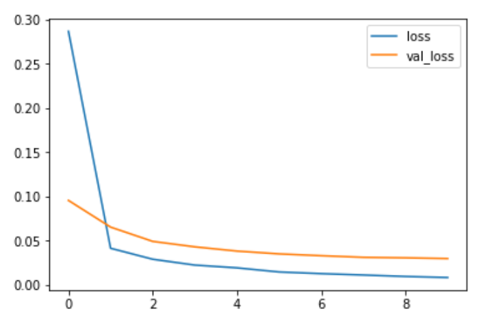
Loss per Iteration plot
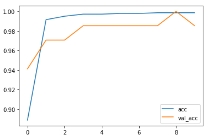
Accuracy per Iteration plot
Now this looks a bit promising,
let's see how it performed.
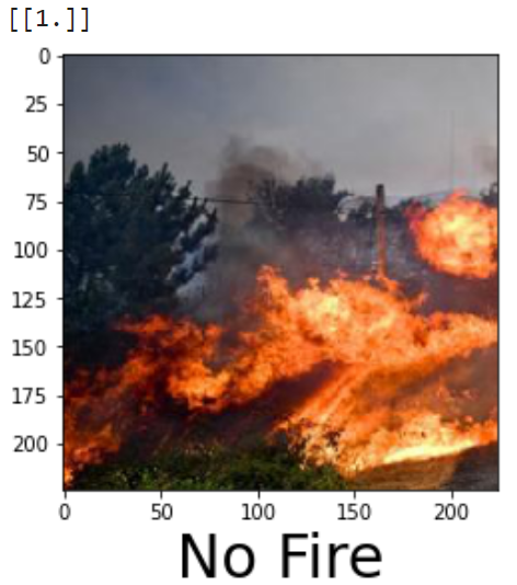
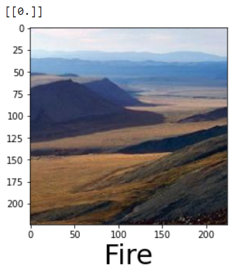
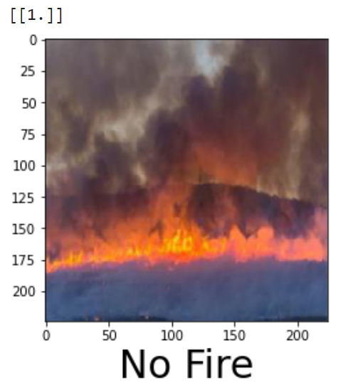
Now this is even more messed up than the previous one 🤣
Let's try one more!
Model 3 Name :- bit/m-r50x1
Feature vector extraction with the BiT-M R50x1 model.
Publisher: Google
License: Apache-2.0
Architecture: ResNet50-v2
Read more on it Here

Loss per Iteration plot
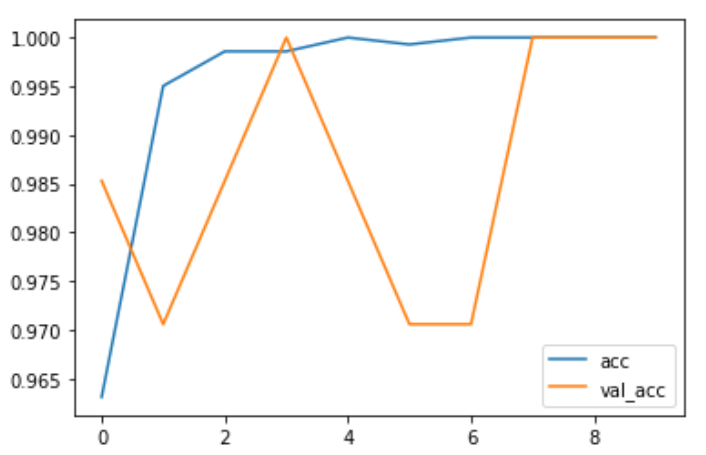
Accuracy per Iteration plot
I know the validation accuracy plot looks messy, but if you look closely, the lowest it gets is still 97%. We can still consider it a great result as it is very close to 100 and it cannot be said as Overfitting or Underfitting.
Let's see how has it performed,

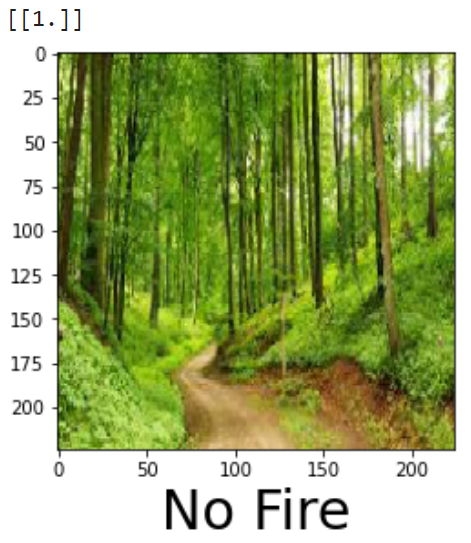
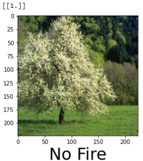
This looks great. We have accomplished our goal. There are more images of predictions which I've not included here. To see those and to try this out yourself please see the GitHub repo for this Project.
GitHub repo : Forest Fire Detection using CNN
. . .
Like , Share if you found this helpful.
I am open to any Suggestions/ Corrections/ Comments so please feel free.
Also , Connect with me on Linkedin
Open to Entry Level Jobs/ Internships as Data Scientist/Data Analyst. Please DM on Linkedin for my Resume for any openings in near future 🤗 🙏


Comments